The Simulation of a Gyroscope
The Gyroscope is a quite fascinating piece of mechanics, though very simple, and for sure everyone in their life has at least once seen and even played with one.
The part is simple, but the phisics behind it is not so intuitive; we are not going to enter into the equations that gouverne the behaviour of a Gyroscope and nonetheless we wanted to simulate it through an FE model.
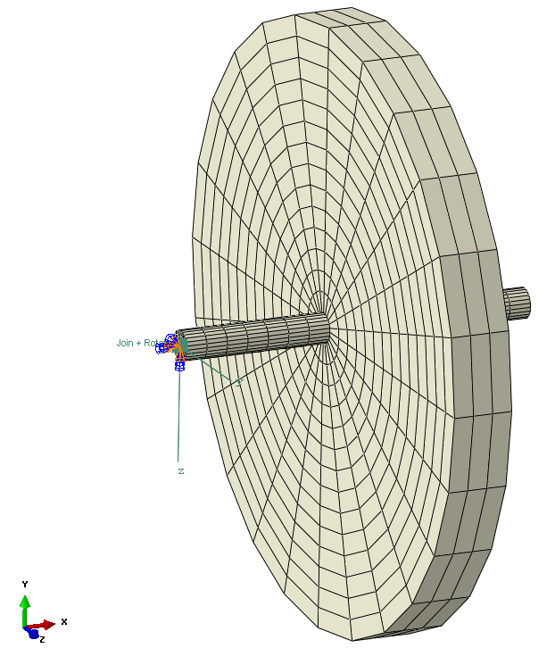
The model is a simple one, as it can be seen from Figure 1; it is basically a steel fly wheel that is constrained at one end with a connector element that allows only the rotations around the three axes, the translations being constrained to ground.
With these boundary conditions, the object is clearly underconstrained and a static solution would very likely exit with an error. So, because the Gyroscope, by its own name, needs to rotate, we know that a dynamic analysis will be required.
Therefore, as a first approach, we try not to impose an angular speed to the object, but just the gravity acceleration along the Y axis and run the analysis. The animation here below shows that what happens is what we expected: the Gyroscope tends to drop.
The second step consisted then in imposing an initial angular velocity around the Gyroscope axis, while the gravity acceleration is still applied. The result of this simulation is shown in the two animations here below, where the behaviour is seen from two different points of view.
We notice two facts:
- The Gyroscope does not drop anymore (Axial Parallelism); the angular speed makes it resisting to the gravity acceleration
- The main axis of the Gyroscope tends to rotate orthogonally to both the rotation vector and the moment generated by the gravity force (Axial Precession)
Those effects have been widely used to stabilize different systems, from aircrafts to ships to steady cameras.
As mentioned, we do not want to enter into the equations (they can be checked on Wikipedia, for example: https://en.wikipedia.org/wiki/Gyroscope): here we just wanted to show that with a proper simulation (which requires the understanding of the phisycs behind the phenomenon), correct results can be achieved. If we thought that by applying the “centrifugal force” (as it is presented from many pre-processor softwares) we could get the same results we would be wrong: to get the gyroscopic effects we actually need to impose a rotation.
One last simulation aspect concerns the type of solution approach for this problem: Implicit or Explicit.
Because the phenomen is not really a high speed one, because we need few instants to check the behaviour (here we have simulated up to 2 s), because the Explicit is conditionally stable (numerical errors tend to sum up), we have decided to use the Implicit approach.
