Back on Buckling
Because we touched the topic in two occasions on these pages (Post Buckling Analysis of a Frame and The Buckling Analysis and Test of a PushRod for a Race Car Suspension) we come back on it with this article, trying to give more insights on the instability of structures.
To make things more understandable, we consider two slender elements (Figure 1 on the left) interconnected with a hinge (Point B); the lower element is restrained to ground with a hinge (Point A – only rotation is allowed), while the upper element has a slider and a hinge (Point C – rotation and vertical translation allowed).
Additionally, between the two elements (Point B), we have a torsional spring with stiffness KT.
As long as the two elements are perfectly aligned, force P can be as big as the cross section of the elements can resist to, let’s say, yielding: the larger the section and the better the material, the bigger P can be.
Nonetheless we know that “perfectly straight and perfectly aligned” are not possible in real world, so a small deviation will always be present, generating the simplified condition shown in Figure 1 on the right, where the angle θ represents the imperfection.
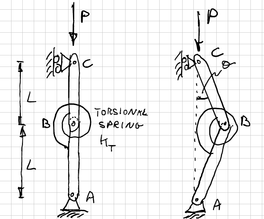
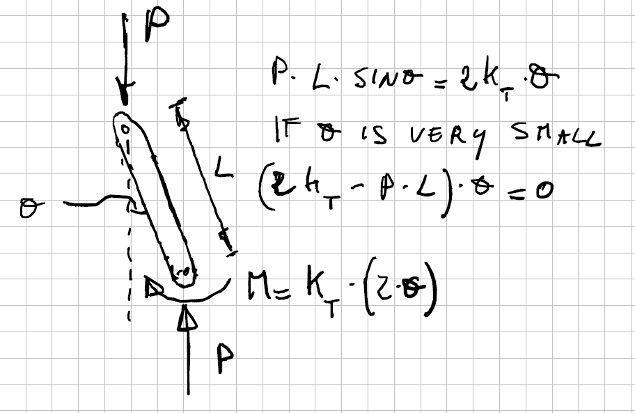
Due to the presence of the torsional spring, the angle θ will generate a moment M between the two elements equal to 2·θ·KT and the FBD (Free Body Diagram) for the upper element is the one shown in Figure 2.
For the structure to be in equlibrium it has to be
P·L·sinθ = 2·θ·KT (1)
Being θ very small, we can assume that sinθ ≅ θ and therefore we can write:
(2·KT – P·L)·θ = 0
The equation above has the trivial solution θ = 0, that represent the unrealistic case of the perfectly aligned elements.
The interesting solution is the one that makes the terms inside the parenthesis equal to zero:
Pcr = 2·KT / L (2)
This is the value of the critical load for this structure. Values of P < Pcr will be equilibrated by the torsional spring.
Values of P > Pcr will still bring the structure to collapse.
Let’s go a little further considering a practical example and assuming L = 100 mm, KT = 10000 Nmm/rad. By using Eq. (2) we get
Pcr = 200 N
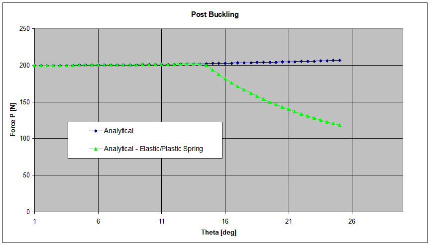
And if we use Eq. (1) to plot P as a function of θ, we get the blue line in the graph of Figure 3. The graph confirms what we know: the structure cannot take loads bigger than Pcr. It also tell us that the force is not suddenly dropping to zero, because the spring will continue to generate a moment proportional to θ.
Nevertheless, also the torsional spring is not “ideal” and in real world it cannot be elastically twisted over a limit angle.
If we assume as an example that the maximum moment that the spring can react is M = 5000 Nmm and we consider that into our Excel sheet, we get the green line in the graph of Figure 3.
Now the force P is actually getting smaller, being the moment constant and having an arm that increases with θ. If we imagine to perform a test on this strucure by applying the load in a “force controlled” way, then we would have a dramatic collapse.
This is the reason why buckling tests are performed with the “displacement controlled” approach: this way it is possible to visually idenify the onset of the instabilization.
Please note that the blue line explains why in the pictures of the articles that we mentioned at the beginning we have constant forces after the critical load has been reached: no limitations to the resisting moment were assumed, exactly like here when the torsional spring is considered to be “ideal”.
Can we simulate this with a Finite Element Model? Of course we can!
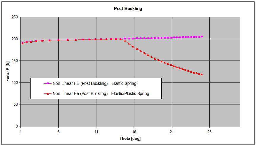
Using a beam model and a connector between the two beams we can simulate both the conditions, i.e. the “ideal” torsional spring and the “limited” one, obtaining the graph shown in Figure 4.
Clearly the calculation has to be non linear due to the large displacements involved and to the limit imposed to the moment that the torsional spring can react.
It is easy to check that, a part some small numerical differences for small values of θ, the FE model behaves as the analytical solution.
It must also be pointed out that a linear buckling calculation on the same FE model has given a value for the critical load very close to the analytical one.
We have used this two element model where we have “concentrated” the instability in a single point, typically Point B, to simplify the speech.
In fact the classical situation or, better said, the one we are more used to see is the one represented in Figure 5.
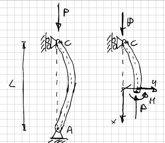
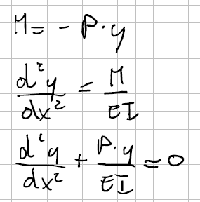
The reasoning is the same: we create the FBD for the structure and write the equilibrium equations, coming to the relationships reported in Figure 6.
As we can see, now we have to solve a second order homogeneous ordinary differential equation, not so difficult but for sure more complex than Eq. (1) and anyway aobve the target of this article.
We can say that its solution leads to the well known equation for the Eulerian critical load of beams:
Pcr = π²·E·I / L²
Post buckling analysis is treated in Chapter 11 of the book “Computational Structural Engineering“.
