The Submodeling Technique

As well known, it is generally a good practice, in a finite element analysis, to perform several iterations
of calculation of the same structure in order to determine what is the best mesh density to obtain reliable results.
In our days the necessity to try and reduce the commitment of the calculation resources
is less felt than some years ago; however in various cases it is useful to employ some tricks in order
to solve models that, in spite of the power of the available systems, could be hard to manage.
In such cases the submodeling technique is there to help us.
The pictures are extracted from Chapter 7 of the book “Computational Structural Engineering“, where the procedure to create and solve a submodel is explained step by step by using a “hand calculation” approach.
The classical bar with a hole in the middle is considered.

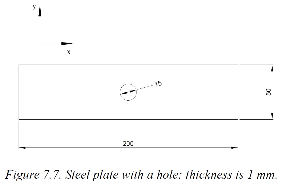
Only a quarter of the plate is modeled, thus leveraging the double symmetry of the structure.

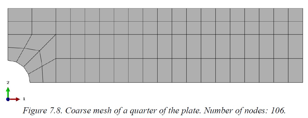
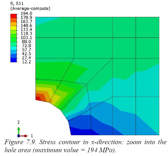
Hand calculations, considering an intensification factor of 2.35 given by the hole, provide a maximum stress value of 235 MPa, while the result from the Finite Element Model shows a maximum of 194 MPa, with an error equal to about 17%. Definitely too much and therefore a mesh refinement is required.

Nevertheless, instead of refining the mesh on the whole model we could create a submodel, by “extracting” the portion of interest and, for example, doubling the number of elements in that region, as shown in the picture below:

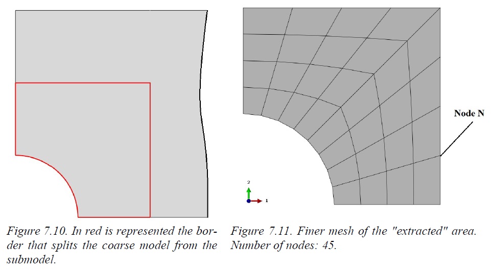
Now the problem is: how do we deal with the boundary conditions to be assigned to the border of the submodel?
The Shape Functions of the element type we are using come to help us. As it is known, Shape Functions are polynomial that describe the displacement of any point inside the element as a function of the displacement of the nodes. Node N in the picture above is a “new” node, i.e. is a node of the finer submodel and it “drops” inside an element of the original, and coarser, model (in this case at half the length of an edge, but this does not affect the general validity of the approach).

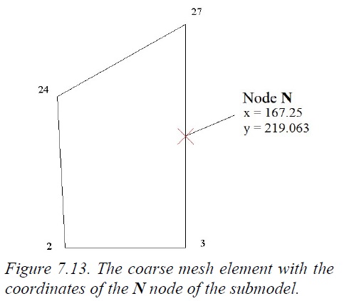
Through the Shape Functions we can then calculate the displacement of the point in the coarse mesh that corresponds to the node N of the finer mesh, By doing this for all the “new” nodes we are able to find the boundary conditions, in terms of applied displacements, to be assigned to the border nodes of the finer submodel. Once this is done, the results obtained from the finer model are shown in the figure here below:

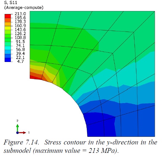
Now the maximum value is 213 MPa, with an error of about 9% with respect to the theoretical values.

Commercial calculation software are able to automatically perform the operations required to find the proper boundary conditions to be applied at the submodel, by just simply selecting the border of the submodel, being this lines (for 2D structures) or surfaces (for 3D structures).

More details in the mentioned book: Computational Structural Engineering!